SW 80m data net experiment - results
This 80m data net took place yesterday at 9pm to about 10:30pm, I have collated the results from the participants and listeners. We have a way to go to get a pan-SW data net, there are things we can do to improve things, but they need some study to work out where to optimise effort.
Understanding 80m propagation
From G0FVJ on the WAB group we learned
Critical frequency.
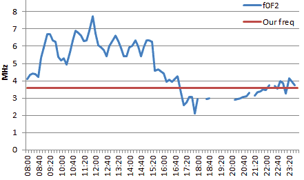
The peak to 7.8MHz coming at 11:45, then an up and down journey to 4MHz by 16:00, and a low of 2MHz at 17:50, then 2.1MHz at 19:45.
So let’s take a look at the data from the Chilton Ionosonde at the Rutherford Appleton Laboratory. Chilton is in Oxfordshire, near Didcot, about 100km from Glastonbury.
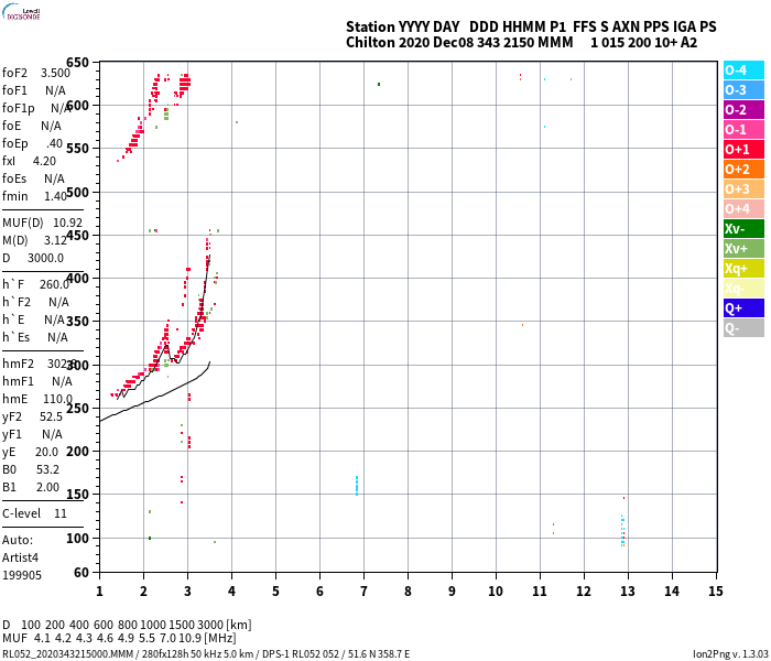
f0F2 dropped below 3.5MHz1 at 17:00 and was out for the count until 21:50, where it hovered around the 3.5MHz mark. This is known as the critical frequency, the frequency above which vertically incident signals pass through the F layer of the ionosphere and are lost to earth-bound stations. This is a first approximation, under some circumstances signals above the critical frequency can be returned by the E layers, which are better known for 2m propagation, see G3YLA’s RSGB Convention video in footnote 1 for more. As you can see in the bottom row on the ionogram, the maximum usable frequency can be higher for shallower angles of incidence, which is why the MUF rises with increasing distance. As an example of this, Tony M0JII decoded SV2BFI in Thessaloniki, Greece at a frequency only about 500Hz lower:
20:54 > Q de SV2BFI SV2BFI SV2BFI
CQ CQ CQ de SV2B RSID:Contestia 16/5ØØ f=1259Hz FI SV2BF
and this was observable on our waterfalls too - FLDigi does not seem to decode two Olivia signals at the same time, but Tony was using Digital Master 780 from Ham Radio Deluxe, which does.
You can see this in action - as the critical frequency started to creep up around 10:20pm I started to receive 2E0GHE from Bristol. I have drawn a 25km circle round Glastonbury on the map to show the broad limit2 of ground wave
TX 22:18Z: 2E0GHE pse go ahead KN
RX 22:18Z: /5lt|RGR your s/n -2.4
RX 22:20Z: RiG: 7300
RX 22:20Z: Ant: EFHV
RX 22:20Z: Pwr:25W
RX 22:20Z: Loc: BristolN!”CH\ f RX 22:20Z: CeMoo PIdX^ 0 TX 22:21Z: 2E0GHE tks fer report your s/n: -3.3 dB much QSB BTU de G7LEE
I don’t have details for the time of the Cheltenham result from G6BHS. Cheltenham is 93km from Glastonbury, so if we look at the ionosonde data then the 100km MUF is shown as 4.1MHz for 21:50, it was marginal at 3.8MHz at 21:00 so I would imagine reception improved as time went by.
Map of stations
Note that locations are approximate, derived from the locator in many cases
How can we improve the results?
I didn’t expect this to be quite this much hard work. Looking at the ionosonde data things we could do to improve the chances of success are:
- Run the net earlier in the day. Around noon is better for NVIS, our experiences with Exercise Blue Ham support this, NVIS propagation starts to drop around 3pm on the 5MHz band
- Optimise for ground wave propagation. This is difficult for many people, and verticals tend to be more sensitive to noise. It is also a question of power, which does not always make friends.
- Turn the bug into a feature - operating between the ends of the Wessex region. Penzance to Glastonbury is 230km, and the MUF rises as the distance increases!
- The VHF packet systems of the 1990s were very successful at regional data networks. The technology is much cheaper now, a Raspberry Pi running DireWolf eliminates the packet TNC and the nod controller.
Other learning opportunities:
Sound the RF paths - we can run WSPR, I have a Raspberry Pi WSPR TX which is reasonably easy to replicate and anyone with a SDR (or a rig prepared to run it 24/7) can collect data from around the region. It is possible to use the Pi and a SDR for RX.
Hone the art of net control. We need more practice in data nets, I found it a struggle trying to stay on top of things, and the latency of the Olivia mode is quite an issue. One thing we did learn was that where skip is bringing in other Olivia signals, leaving RXID enabled can mean you get pulled off the frequency of the net you are in.
Signal reports
| Call/Name | loc (PWR) | Notes | G7LEE | G4JJP | G5FM | G8DMN | 2E0GHE | ||
|---|---|---|---|---|---|---|---|---|---|
| G7LEE / Richard | IO81pd (12) | horiz FW loop QRM S7 | -4.2 | 16.7 | 2 | -8 | |||
| G4JJP / Richard | IO81re (25) | EFHW invL | -11.8 | ||||||
| G5FM / Martin | IO81pd (10) | in V 60m dip | |||||||
| G8DMN / Simon | IO81rd (30) | 1.4 wave in V @ 6m | -5 | 8 | -9 | ||||
| 2E0GHE | Bristol (25) | EFHW much QSB (G7LEE) | -2.4 | ||||||
| Listeners | |||||||||
| M6MQB / Matt | IO81pd | ||||||||
| 2E0FNT / Matt | IO81pd | ||||||||
| M0JII / Tony | copy | copy | copy | copy | copy | ||||
| M7AHJ | IO81ma | S9 +40 | no copy | no copy | no copy | no copy | mo copy | ||
| G6BHS | Cheltenham | sporadic decodes |
There are practical problems running 80m HF in an urban area, noise tends to rise towards lower frequencies.
-
The RSGB has a good Convention video by Jim Bacon, G3YLA on how to interpret ionosonde data for local nets, relevant section starts here ↩
-
The ARRL seem to indicate ~55 miles for ground-wave prop on 80m, but I was using a horizontal loop rather than a vertical, so I am not optimised for GW. The ARRL estimate is shown in orange, I have difficulty in believing this, though perhaps running a big gun station at the US legal limit can do it ;) ↩